Excel uses a system of rows and columns to help users organize information within a document. Excel offers its users an abundance of different features to allow for better data management within the program. One such function that users could find useful to help manage content better is to freeze rows and columns simultaneously. However, Microsoft Excel hasn’t made it easy for users to freeze the top row and the first column together. Learn how you can freeze the first column and the top row together.
While Excel offers a “Freeze Panes” feature, which allows users to freeze the first row and column individually, you cannot freeze both of them together. However, you can work around the “Freeze Panes” section to simultaneously freeze the top row and first column.
Instead of just going to the “Freeze Panes” section and just trying to “Freeze Panes” normally, you need to select the cell under the first row and after the first column. You can then use the “Freeze Panes” method to simultaneously freeze the top row and first column. Users who are often frustrated that they cannot freeze the first row and column simultaneously can miss this hidden step. However, if you use the method shown here, you can freeze them first row or first column simultaneously.
How to freeze top row and the first column at the same time in Excel:
- Firstly, open your Excel document.
- From there, click on “View.”
- Then select the cell under the first row and after the first column.
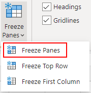
- Now click on the drop-down next to “Freeze panes.”
- Select “Freeze panes” to complete the process.
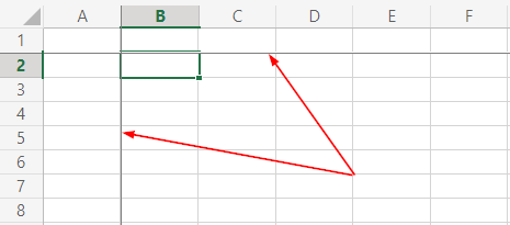
Upon completing the steps above, the first row on the first column of the document will freeze in place. You can move around the document without the first row or the first column moving and disappearing from the view pane. Users forget that the “Freeze panes” option requires you to select a cell as a marker. Selected cells act like a corner which Excel uses to create the freeze pane. Anything above the cell that you have selected and anything to the left side of the cell will be frozen in place when the steps are complete. You will know that both the row and column are frozen because there will be a thick black line indicating that those cells are frozen, as shown below.
We’ve also created a video to help guide you through the steps:
![]() Excel users can add
Excel users can add ![]() Ablebits to gain access to more than 70 professional tools!
Ablebits to gain access to more than 70 professional tools!
An in-depth guide on how to freeze the top row and the first column at the same time in Excel
The Microsoft Excel UI can be quite difficult to follow; you may require the assistance of an in-depth guide to help. The in-depth guide features screenshots that will allow you to navigate the process and better understand what the actual end goal will look like. For instance, if you need to know what the frozen panes look like at the end of the process, you can use the screenshots to help. Screenshots provide a far more effective way for you to follow through the process than just the text provided. We will also provide some in-depth analysis to complement the screenshots; you can use this for further information.
- Firstly, open your Excel document.
This can be a current document you are working on where you need the first row on the first column of information frozen, or you can launch a new document to test the process. Either way, make sure your document is open to continuing ahead.
- From there, click on “View.”

There will be a menu option to select all the different tools and functions within the program. From here, you need to select the option for “View.”
- Then select the cell under the first row and after the first column.
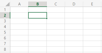
As you can see from the screenshot above, the cell I selected is B2. Cell B2 is under the first row and directly after the second column. Now when I proceed with the steps ahead and begin to put the freeze panes, you will have the freeze panes automatically set in place.
As stated above, the freeze frame will be applied to the row above on the column on the selected left side of the cell. All those rows and columns will be frozen when you continue with the steps ahead.
- Now click on the drop-down next to “Freeze panes.”
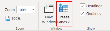
Next to the option for “Freeze Panes,” there will be a drop-down; you need to click on this to proceed with the steps ahead. Freeze panes are essentially the option you can use to freeze the top row and side column depending on what is required. Here, you can freeze only the top row and the column if necessary. However, if you have followed the steps above and selected one of the cells, you can freeze both the top row and side column simultaneously.
- Select “Freeze panes” to complete the process.
A row and side column will be frozen once the steps above are complete. Microsoft has made it in such a way that you need to select the cell before you proceed to freeze the top row and first column at the same time. Many users often overlook this, and therefore they can’t freeze the column and row simultaneously. You need to consider these additional steps before you use the Freeze Panes option. You can select whichever cell is necessary, and any rows above and column towards the left will be frozen and will not move when you continue to use the sheet.

Conclusion
Thank you for reading our content and how you can freeze the top row and first column at the same time. We have given you the steps on how you can freeze the top row and column at the same time within the program. Many users overlook the essential step of selecting the cell under the first row and after the column to freeze both of them simultaneously. However, once the steps above are complete, you will have successfully managed to freeze both column and row simultaneously. If there are any issues you come across when following the steps above, simply drop a comment below we will address them.