How to grey out unused areas of a worksheet: Excel

Key Takeaways

The simplest way to grey out unused areas of a worksheet is to fill all the cells with a grey background, select your used cells, and fill them with “No Fill.” [More…]

Alternatively, to retain any background formats, click the first row header under your work area, press Control/Command + Shift + Right, and fill the selected rows with a grey background. Then, click the first column header to the right of your work area, press Control/Command + Shift + Right, and fill the selected columns with a grey background.

Greying out worksheet areas can improve the overall aesthetic and highlight only the important rows and columns. There are several methods to achieve the effect, which we will look at in detail within this blog guide.

How to grey out unused areas of a worksheet in Excel:

Firstly, open your Excel worksheet.
Click the triangle icon in the top left corner to select the entire sheet.
Click the down arrow next to the “fill color” icon and choose a grey color.
Select the top left cell in your worksheet.
Press Control/Command + Shift + Right arrow.
Press Control/Command + Shift + Down arrow.
Click the down arrow next to the “fill color” icon and choose “No Fill.”

Optional – protect the sheet so that greyed cells cannot be edited:

Click the top left cell in your worksheet.
Press Control/Command + Shift + Right arrow.
Press Control/Command + Shift + Down arrow.
Right-click any highlighted cell and select “Format cells” (or press Command/Control + 1).
Go to the “Protection” tab at the top of the dialog box.
Uncheck the checkbox next to “Locked.”
Click the “OK” button.
Click on “Review.”
After that, click on “Protect Sheet.”
Under “Allow users of this sheet to,” ensure the option for “Select locked cells” is unchecked.
Add a password to protect and unprotect the sheet.
Finally, click “OK.”

Get Excel for just $6.99 per month from the Microsoft Store!

The greyed-out cells will not be editable if you complete the optional steps

We’ve also created a video to help guide you through the steps:

How to grey out unused areas of a worksheet in Excel

We have provided several solutions in this guide for greying out areas of an Excel worksheet. You can use the links below to jump to the most relevant solution or try each one to find the best fix.

Solution 1: Fill the background color of unused cells.
Solution 2: Reduce the height and width of unused cells.
Solution 3: Use page breaks.
Solution 4: Hide unused cells.
Solution 5: Use third-party tools.

Solution 1: Fill the background color to grey out unused areas of a worksheet in Excel

Firstly, open your Excel worksheet.
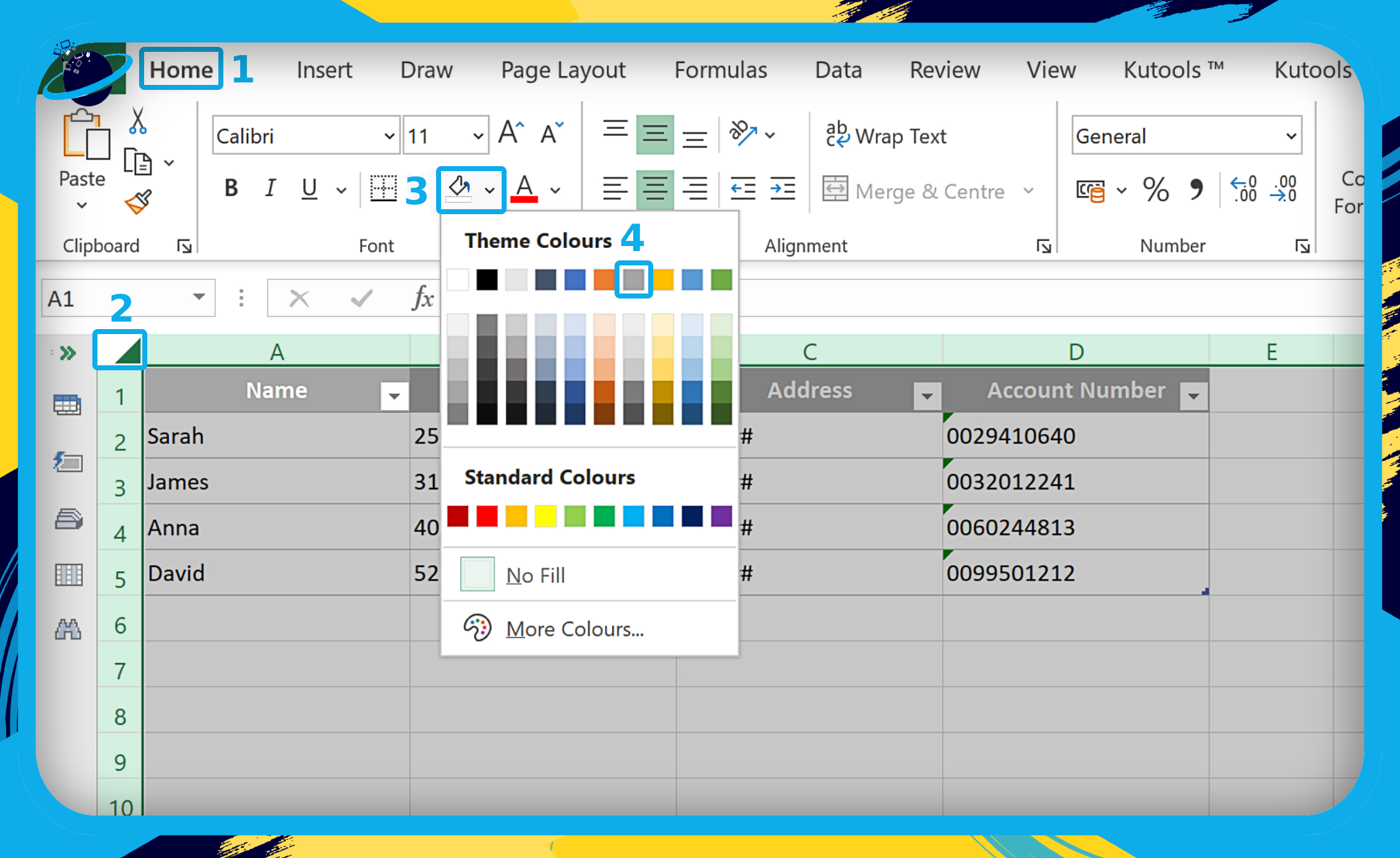
Go to the “Home” tab in the top menu. (1)
Click the triangle icon in the top left corner. (2)
Click the down arrow next to the “fill color” icon. (3)
Then choose any shade of grey. (4)

Note: cells with filled backgrounds will lose their color when using this method. To retain formatting:

Click the first row header under your work area, press Control/Command + Shift + Right, and fill the selected rows with a grey background.
Then, click the first column header to the right of your work area, press Control/Command + Shift + Right, and fill the selected columns with a grey background.

Select the top left cell in your worksheet and select your used cells. (1)
- Press Control/Command + Shift + Right arrow.
- Press Control/Command + Shift + Down arrow.
Click the down arrow next to the “fill color” icon. (2)
Then choose “No Fill.” (3)

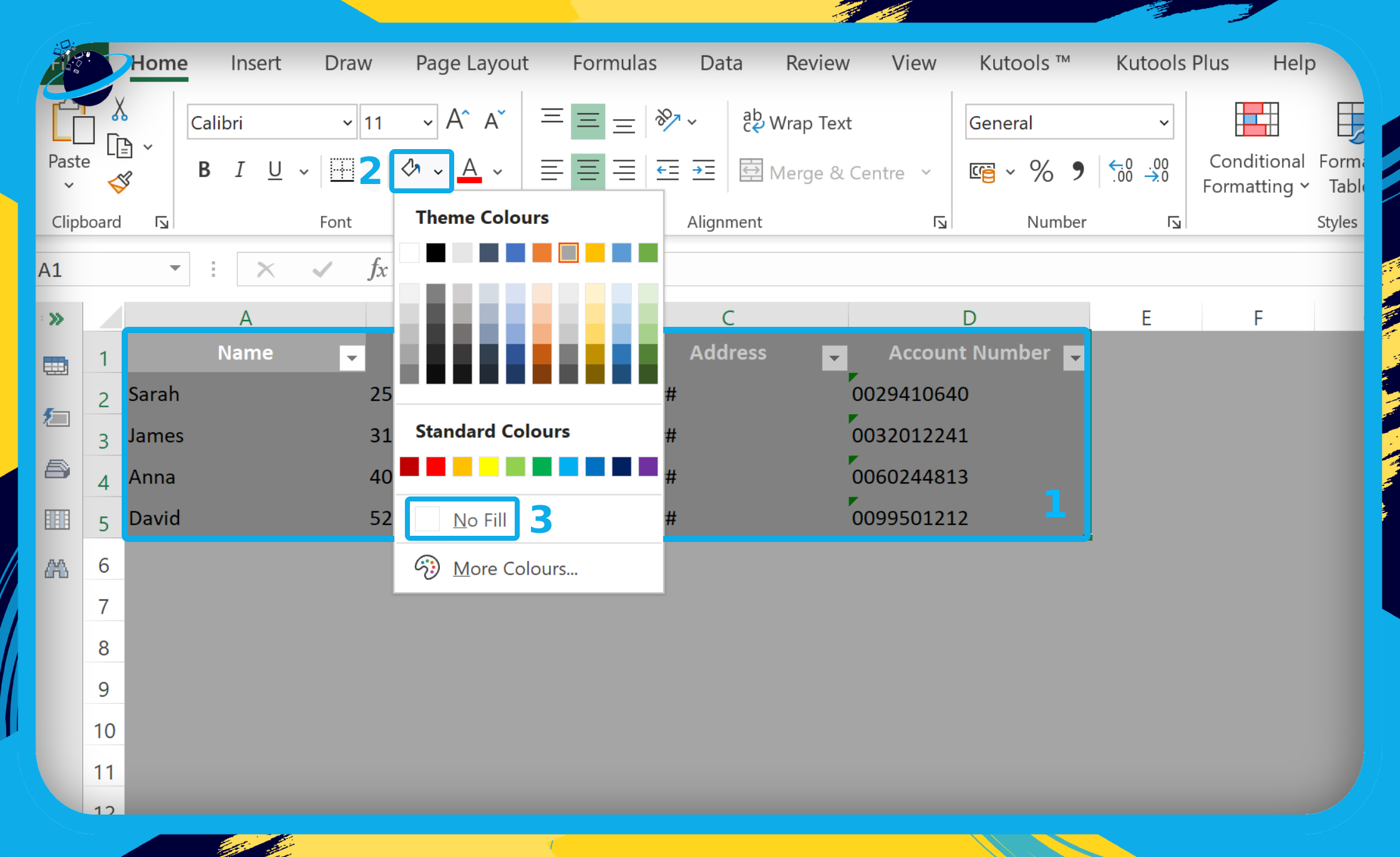
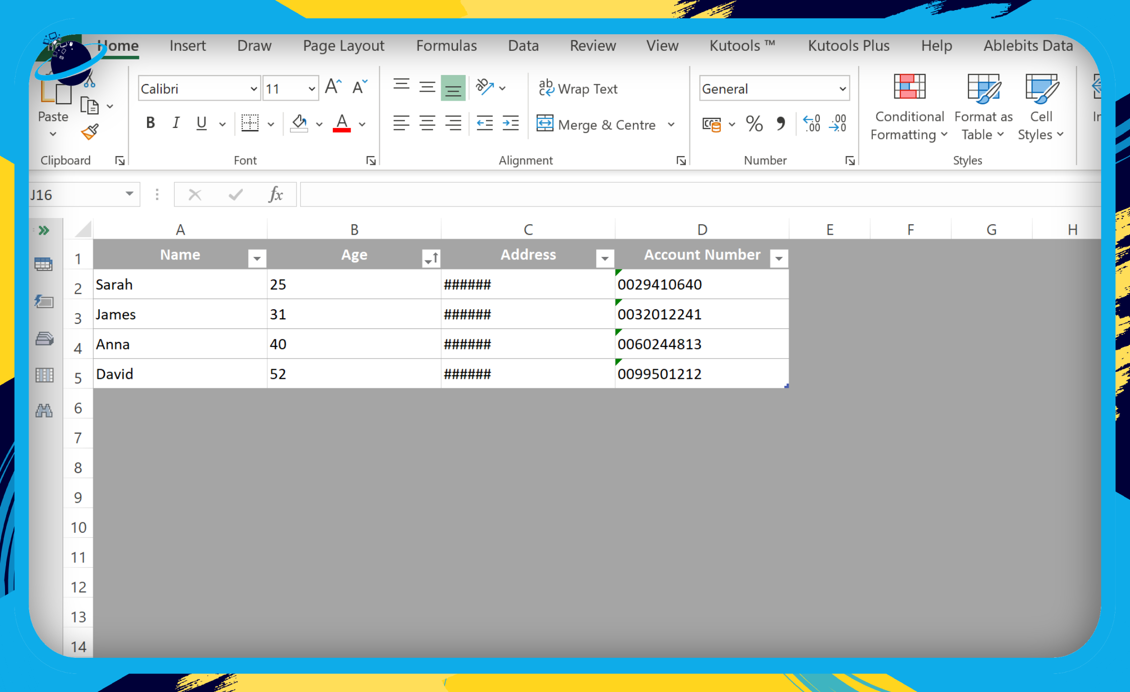
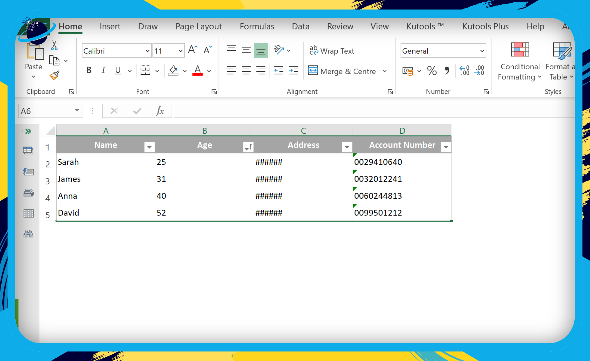
The result shows the unused rows and columns greyed out in the worksheet:

Optional – protect the sheet so that greyed cells cannot be edited:

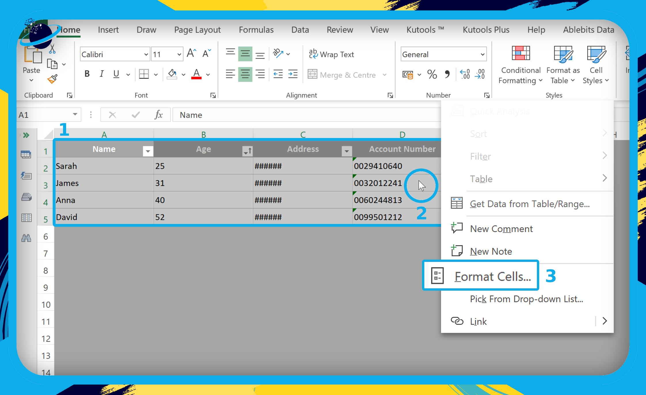
Select the top left cell in your worksheet and select your used cells. (1)
- Press Control/Command + Shift + Right arrow.
- Press Control/Command + Shift + Down arrow.
Right-click any of the highlighted cells. (2)
Select “Format cells” from the popup menu. (3)
- Alternatively, press the Control/Command + 1 keys.

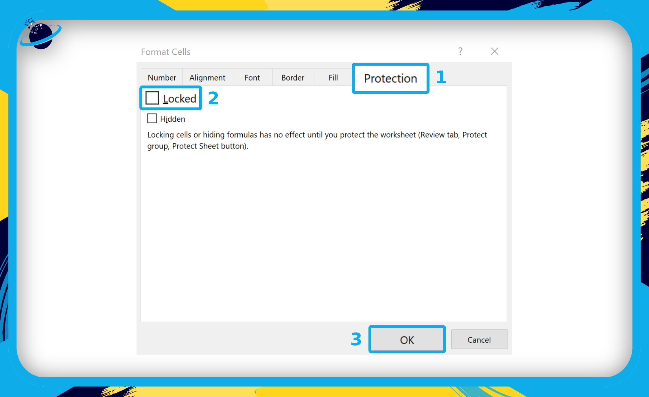
Go to the “Protection” tab at the top of the “Format Cells” dialog box. (1)
Uncheck the box next to “Locked.” (2)
Then click the “OK” button. (3)

Note: by unchecking the “Locked” checkbox, all the currently selected cells will be unlocked and editable, even if you protect the worksheet.

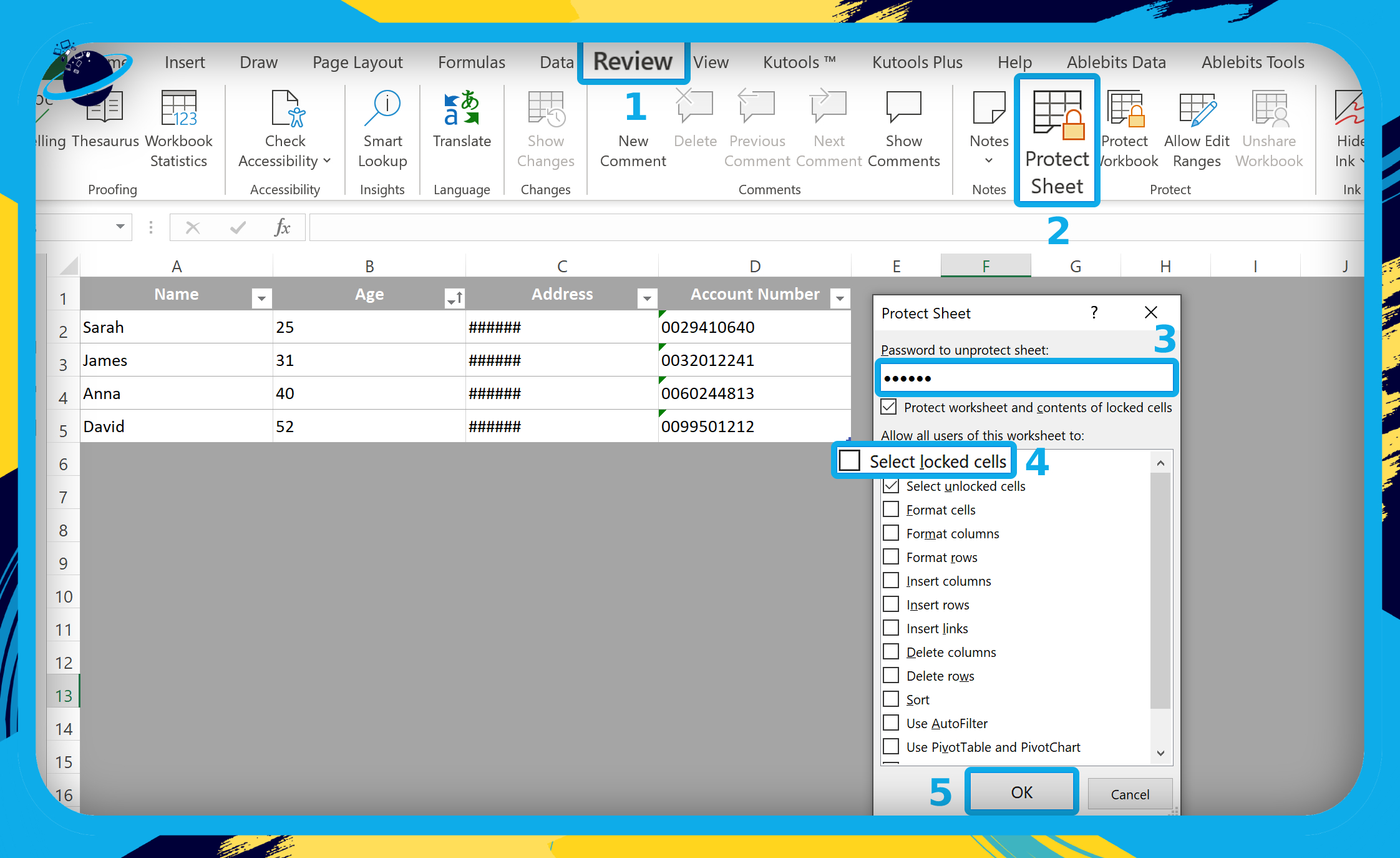
Next, go to the “Review” tab in the top menu. (1)
Click “Protect Sheet.” (2)
Enter a password to protect and unprotect the worksheet. (3)
Uncheck the box next to “Select locked cells.” (4)
Then click the “OK” button. (5)

Re-enter your password when asked to confirm, then click “OK.”
You will no longer be able to select or edit the greyed-out area.
To undo the change, click “Unprotect Sheet” in the ribbon.
Then enter your password and click “OK.”

Solution 2: Reduce the height and width of cells to grey out unused areas of a worksheet in Excel

For this solution, we will set the row height and column width of unused cells to 0. Doing so will effectively hide the unused cells from view and grey out unused areas in your Excel worksheet.

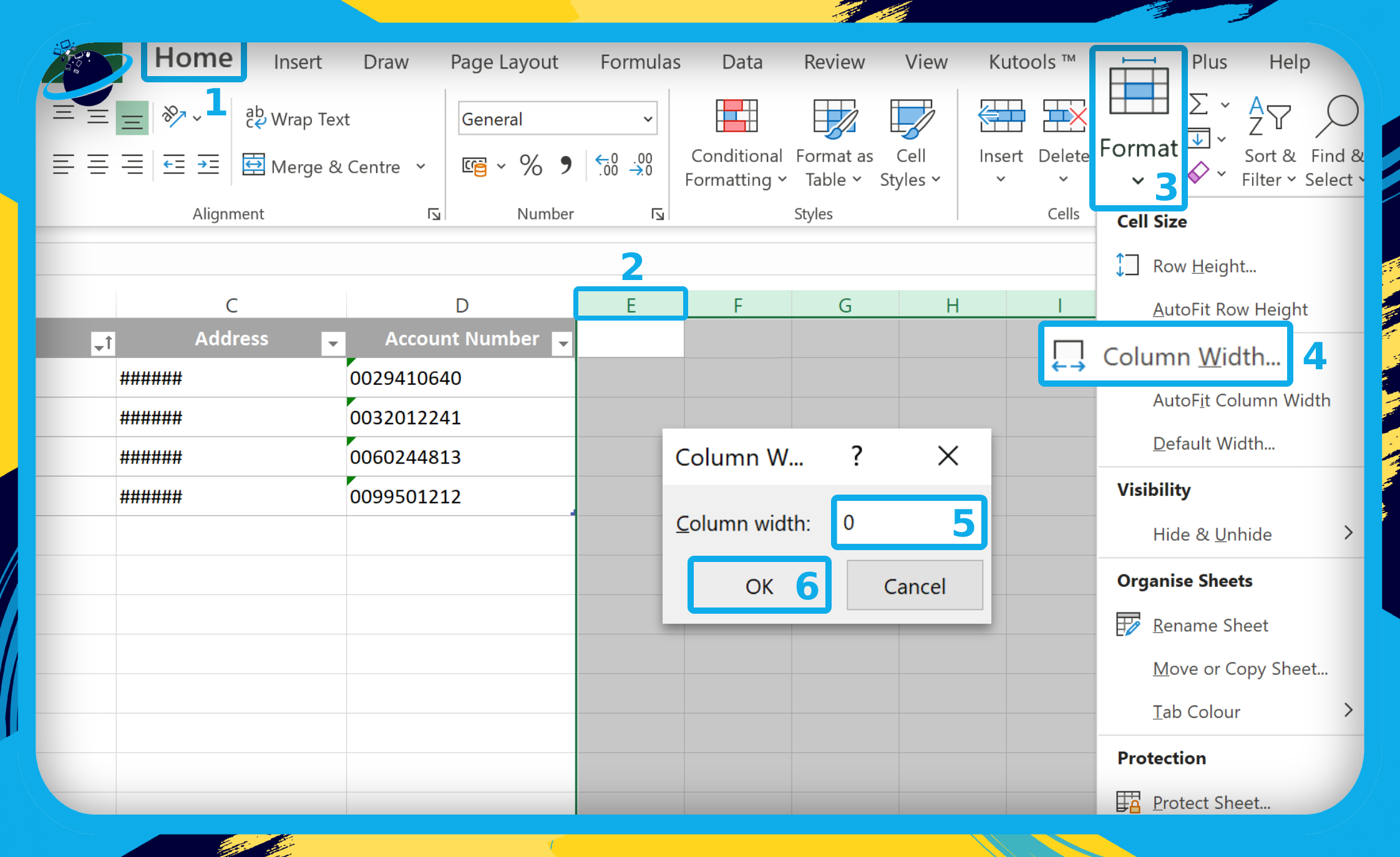
Go to the “Home” tab in the top menu. (1)
Select the first column header to the right of your working area. (2)
- Press Control/Commend + Shift + Right to select all columns to the right.
Click “Format” in the ribbon. (3)
Select “Column Width…” from the dropdown menu. (4)
A small dialog box will appear.
Type “0” in the “Column width” box. (5)
Then click the “OK” button. (6)

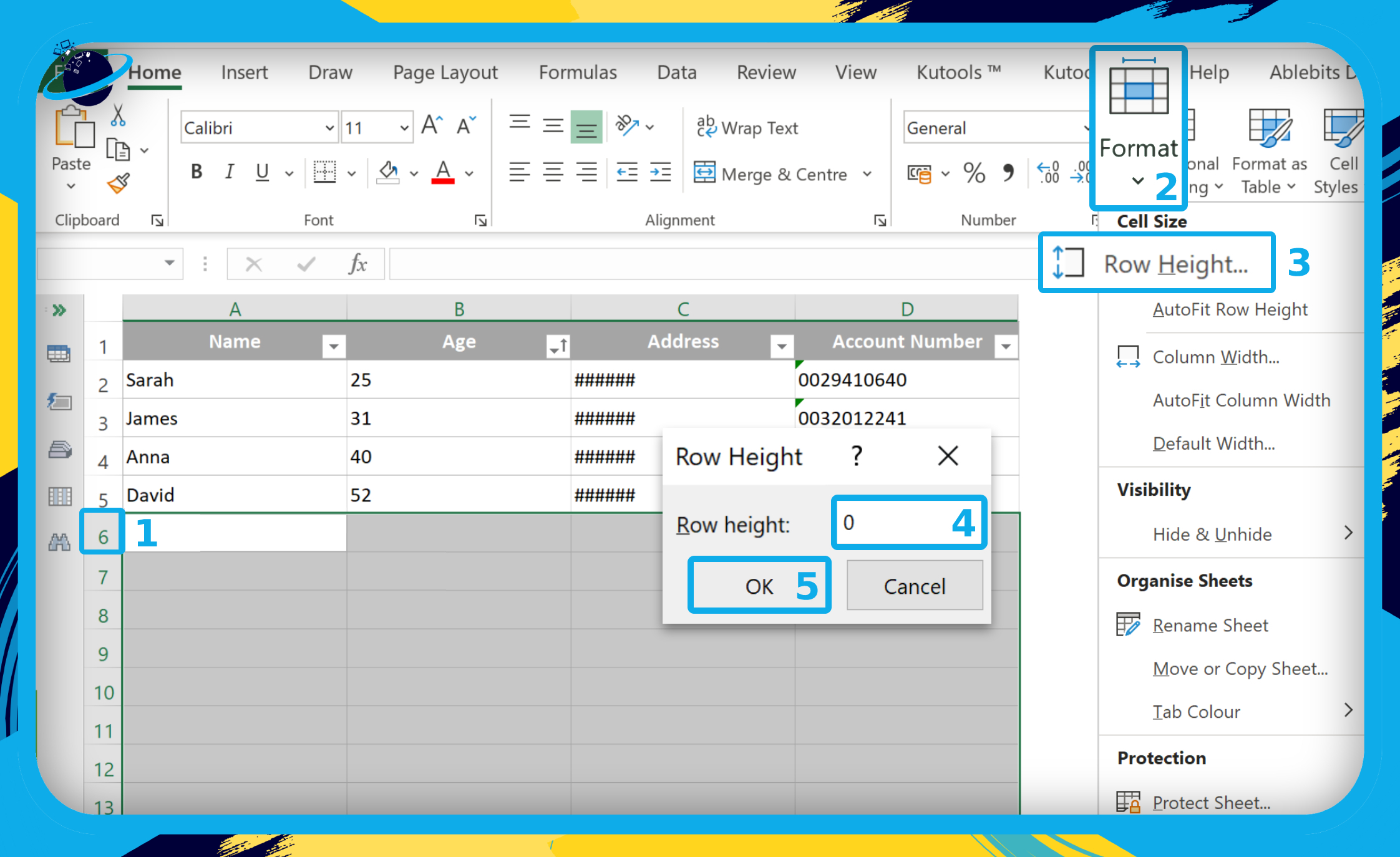
Next, select the first row header below your work area. (1)
- Press Control/Command + Shift + Down to select all rows below.
Click “Format” in the ribbon. (2)
Select “Row Height…” from the dropdown menu. (3)
A small dialog box will appear.
Type “0” in the “Row Height” box. (4)
Then click the “OK” button. (5)

The result shows that the cells to the right and below the work area are now hidden.

To undo the change, click the grey triangle icon in the top left corner.
- The triangle icon will select all cells, including those which are hidden.
Then go to “Format” and change the “Row Height” and “Column Width.”

Solution 3: Use page breaks to grey out unused areas of a worksheet in Excel

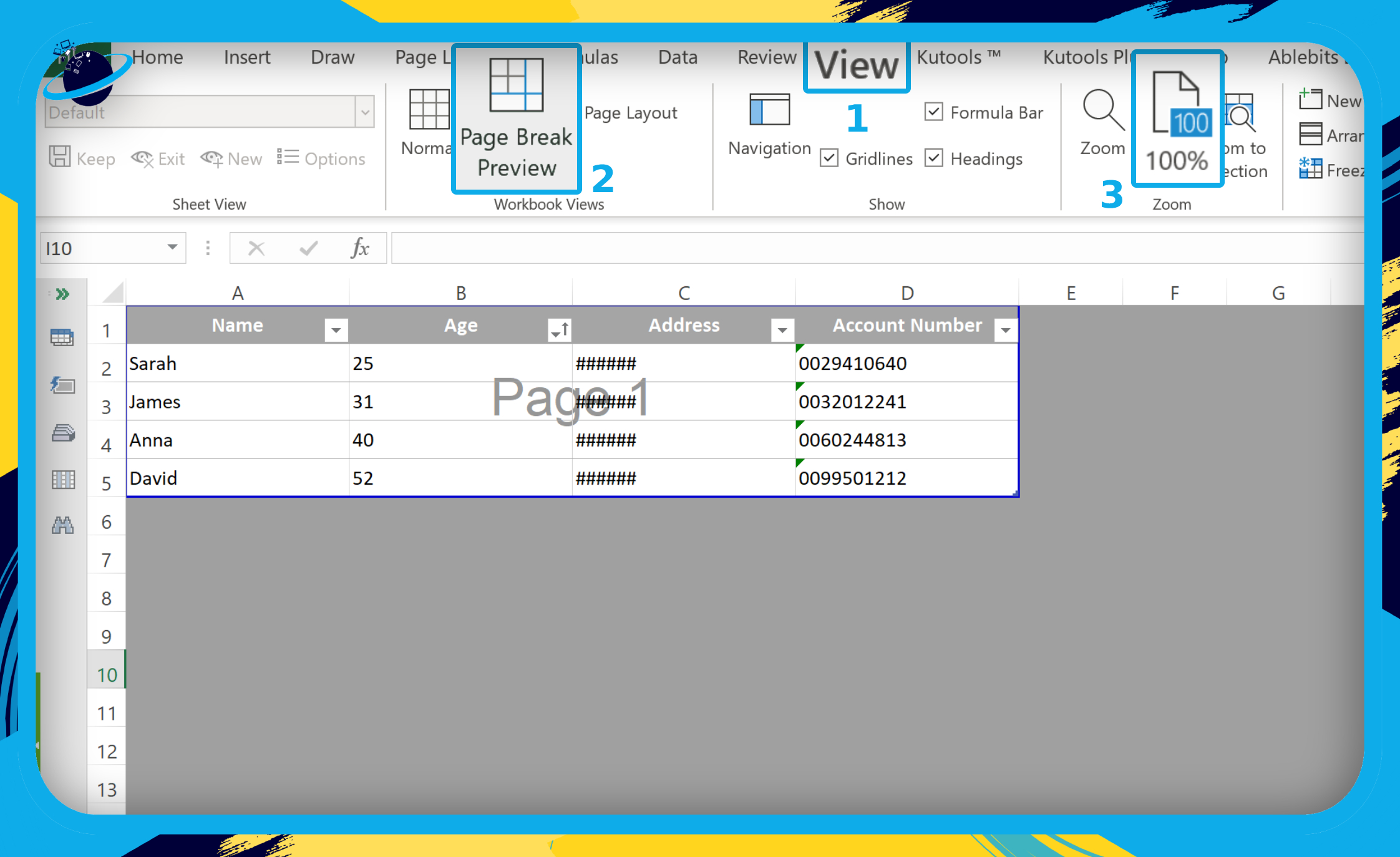
The quickest way to grey out unused columns and rows in Excel is to use the page break preview. Unfortunately, the page numbers will appear on top of your work area as a watermark, which may obscure certain cells.

Go to the “View” tab in the top menu. (1)
Click on “Page Break Preview.” (2)
Then click on “100%” to zoom back in. (3)

To undo the change, click on “Normal,” located to the left of “Page Break Preview.”

Solution 4: Hide cells to grey out unused areas of a worksheet in Excel

Hiding your unused cells is another simple way of greying out the unused areas of a worksheet. The effect will be similar to reducing the row height and column width as described in Solution 2.

Go to the “Home” tab in the top menu.
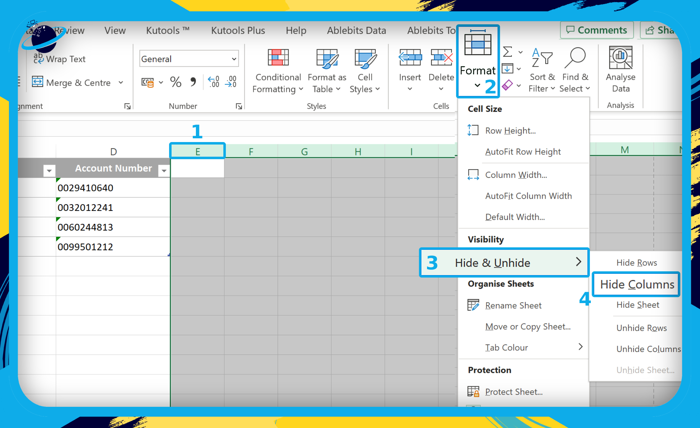
Select the column header directly to the right of your last used column. (1)
- Press Control/Command + Shift + Right to select all columns to the right.
Click on “Format” in the ribbon. (2)
Go to “Hide & Unhide” in the dropdown menu. (3)
Then select “Hide Columns.” (4)

Select the row header directly below your last used row. (1)
- Press Control/Command + Shift + Down to select all rows below.
Click on “Format” in the ribbon. (2)
Go to “Hide & Unhide” in the dropdown menu. (3)
Then select “Hide Rows.” (4)

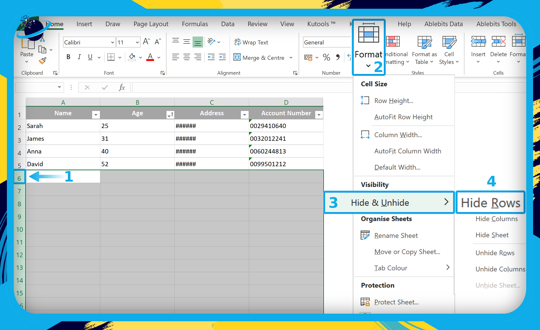
The result shows that the cells to the right and below the work area are now hidden.

To undo the change, click on “Format” in the ribbon.
Then go to “Hide & Unhide” >
- “Unhide Rows“
- “Unhide Columns“

Solution 5: Use third-party tools to grey out unused areas of a worksheet in Excel

For this solution, we will look at Kutools — one of the most popular add-ins for Microsoft Excel — with over 300 additional tools and options to simplify your tasks. The particular tool we’re interested in is called “Set Scroll Area.”

300+ Professional tools and options
$49.00 one time payment or 30-day free trial.

Get Kutools

First, download Kutools.
Once installed, you will see two new tabs in the top menu: Kutools ™ and Kutools Plus.
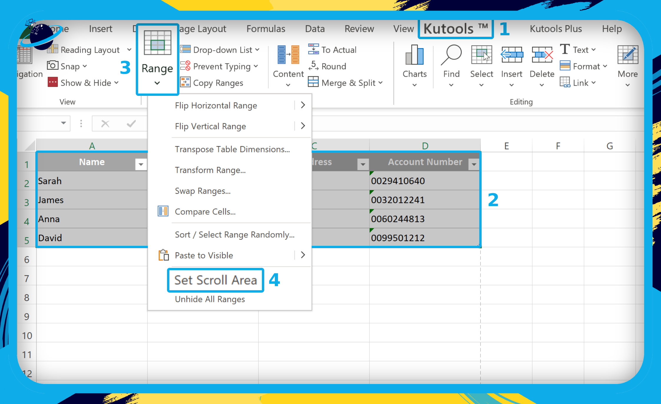
Go to Kutools ™. (1)
Select the cells you want to keep in your work area. (2)
Click on “Range” in the ribbon. (3)
Then select “Set Scroll Area” from the dropdown menu. (4)

The result shows that the unused cells have been hidden.

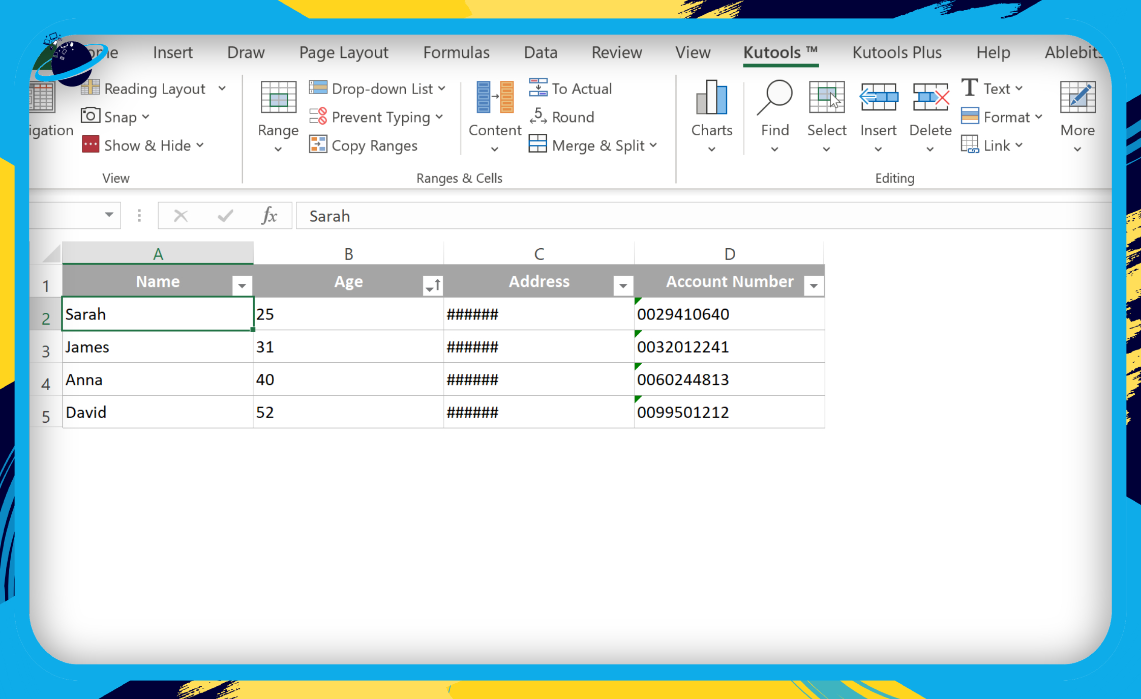
To undo the change, click on “Range” again and select “Unhide All Ranges.”

Frequently Asked Questions (FAQ)

How do I make an Excel cell inactive?

A grey cell is not necessarily inactive. To make an Excel cell inactive, start by selecting all cells in your workbook by clicking the triangle icon in the top left corner.

Right-click any selected cell and go to “Format Cells.”
Go to the “Protection” tab in the dialog box.
Uncheck the box next to “Locked” and click “OK.”
Select the cells to make inactive.
Right-click any selected cell and go to “Format Cells.”
Go to the “Protection” tab in the dialog box.
Check the box next to “Locked” and click “OK.”
Go to the “Review” tab at the top and click “Protect Sheet.”
Add a memorable password.
Uncheck all boxes except for “Select unlocked cells.”
Click the “OK” button.
Re-enter your password and click “OK” again.

How do I mask data in Excel spreadsheet?

To mask data in Excel, select the cells to mask, right-click, and select “Format Cells” from the popup menu. Then, in the “Custom” category, enter ;;;** in the “Type” box and click “OK.” The data will still be viewable in the value bar. To prevent that, make the masked cells inactive by following the steps for “How do I make an Excel cell inactive?” in the section above.

Conclusion

Greyed-out cells in Excel are used to highlight the work area and improve the overall aesthetic of the worksheet. However, grey cells can still be used to contain data. That’s why coloring the background of unused cells is the best solution if you want to add additional rows or columns to the worksheet.

If you don’t want to add any additional rows or columns and you want all unused cells to be inactive, the best solution is to hide unwanted rows and columns (solution 4) or reduce their height and width to 0 (solution 2).

Thanks for reading.