Shortcuts on software such as Microsoft Excel refers to users being able to navigate to different functions within the program with the help of keyboard shortcuts such as pushing select keys to copy content and same with pasting, rather than having to navigate to the functions themselves, it saves a lot of time and improves productivity rates. Got a task list on Microsoft Excel and you quickly want to apply a tick to a completed task? Well, there’s a shortcut for it — follow through this blog as we give you more information on how to apply a tick using shortcuts.
Below is a step-by-step guide on how to apply a tick using shortcuts in Microsoft Excel, follow through as we provide the steps necessary to conduct the following process which will include an in-depth guide as well as a shallow guide to allow you to add a tick in Microsoft Excel.
- Firstly, open your Excel document.
- Now select the cells you want to apply a tick to.
- From there click on the “Font” dropdown.
- Scroll down and select the “Wingdings 2” font.
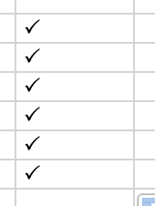
- Finally, once the font is selected, simultaneously press “Shift + P”.
That’s it, following the steps above will allow you to apply a tick using shortcuts quickly on Microsoft Excel. The font has another set of character keys when you press the shift key, once you press shift you will be able to access the additional keys and the font key for the tick symbol is “Shift + P”.
A tick symbol, also known as a check symbol or checkmark, is a particular symbol (✓) that may be put in a cell to communicate the idea “yes,” such as “yes, this response is correct” or “yes, this choice applies to me.” The cross mark (x) is sometimes used for this purpose, but it is more commonly employed to signal incorrectness or failure.
This is the tick symbol that allows for users to effectively check off certain tasks in Excel, the classic layouts are represented in the outcomes above. The illustration on the left shows the Task followed by the outcome which in this case refers to the completion of that particular task. I used the method above to apply the font to the Outcome column and once this was applied I can now easily apply ticks without having to navigate over to the symbol section. I pressed “Shift P” for the tick symbol, “Shift O” for the cross symbol. To apply the symbol with a box around it press the following keys. Press “Shift R” for a box with a tick inside it and press “Shift T” for a box with a cross symbol inside.
In-depth step-by-step guide – What is the shortcut for a tick in Excel?
Below is a more in-depth guide on how you can apply a tick on Excel using shortcuts, follow through for more information on how you can apply a tick on Excel using shortcuts.
Step by step breakdown[with screenshots]
- Firstly, open your Excel document.
The process is the same for both Mac users and Windows OS users, open the application to access your document where you need to apply the tick mark.
- Now select the cells you want to apply a tick to.
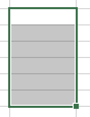
Column F is where the font will be applied, when you select it and apply the font to it, you will be able to proceed by adding a tick to it.
- From there click on the “Font” dropdown.
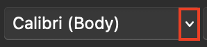
The font dropdown in the menu bar will allow you to access the fonts that you need to apply to attain the ticks in Excel.
- Scroll down and select the “Wingdings 2” font.

Once you have entered the font section of the dropdown, scroll down until you find, Windings 2 font, click on it to apply the final font. You must make sure that only this particular font is applied to the cells, if any other font is applied it will not net a result for the ticks, once applied you will be able to proceed with the following steps which actually involve applying the ticks to the cells.
- Finally, once the font is selected, simultaneously press “Shift + P”.
Finally, once you have applied the font correctly, you will be able to proceed by adding a tick by pressing “Shift + P”. You can alternatively use “Shift + O” to apply across in the formatted cell, just remember that you need to apply the correct formatting before you proceed.
That’s it; by following the methods above, you’ll be able to swiftly apply a checkmark to Microsoft Excel utilizing shortcuts. When you hit the shift key, you’ll be able to access a new set of character keys, and the font key for the tick sign is “Shift + P.”

What’s the need to use checkmarks in Excel?
Checkmarks in Excel are a great way to approve and sign of a task completed in Excel, if you have some goals set you can great a table with each element of the goal and as you complete them, you can use the method above to apply a tick to that particular goal.
If you have some business-related goal such as fulfilments required by a marketing department or finance department, you can use the method above to create a table for all the goals and once you apply the correct format you can apply the tick or cross mark in Excel.
Conclusion
Thank you for taking the time to read our resources; please contact our team to let us know how it went if you followed the advice or if you have any further questions about the issues covered in this blog. If the problems remain after following the measures indicated above, please contact our knowledgeable team at any time, and we will assist you in addressing the recurring error that is causing problems in your workplace. Please contact our team by leaving a remark, and we will take care of the problem. Other people who are having similar issues will be able to get their issues resolved as well.