You’re working on an Excel spreadsheet — say something like a schedule of some sort which has a column of dates to help schedule your days in the most effective manner. However, you realize your dates are in the wrong format set for a country that is not yours. Dates are saved as integers in Excel; the first date is January 1, 1990. You can view the date that positive numbers reflect by formatting them in one of the date formats. This issue is common and can baffle a few people. There could be multiple reasons why it may seem off, from a human error to errors persisting within the tool. In this blog, we will cover ways you can fix the date formatting in Excel so it shows dates for your region or your preferred date format.
I have configured a list of potential options you can use to help configure your Excel sheet so that it shows you the dates in the correct format. Follow through to see how you can change the date formatting to suit your preferences.
- Get Excel for just $6.99 per month from the Microsoft Store!
Use the default date formatting
The default formatting section is where cell formatting can be altered to suit a specific format. If you have prices on you can set the formatting to currencies if you have dates you can set it to date. This opens a huge range of different possibilities for you to customize your Excel experience. You can better organize content rather than just having numbers you can set it to work with many different functions.
Step by step process – Use the default date formatting
- Firstly, open your Excel document.
- Now select your dates column.
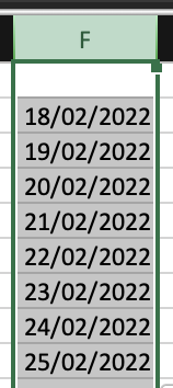
In this case, my date column is the column marked “Date completed”.
- Select “Home”.

- In the “Numbers” section click on the dropdown.
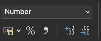
- After that click on “More Number Formats”.

Excel uses logic to detect your existing data formats, as well as a few related date formats or obvious date formats where it might infer it’s a date. It will format your pasted-in data as a date in the cell it is in if it can match it to a valid date.
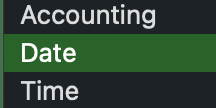
- Select “Date”.
- Select the “Locale (location):” to be your preferred date format.
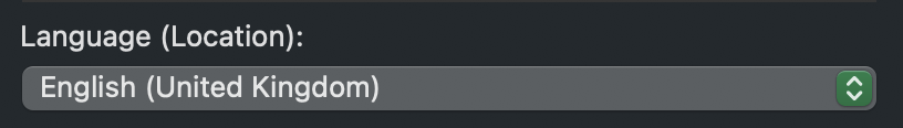
- Then press “OK”.

Note that if you have manually set or altered the dates against what the formatting is set to, you will need to edit the dates again to ensure they are organized in the correct format.
When you type “2/2” into a cell, Excel interprets it as a date and formats it according to the Control Panel’s default date settings. It might be formatted as “2-Feb” in Excel. The default date format in Excel will change if you modify your date setting in Control Panel. You may change the date format in Excel if you don’t like the usual one, such as “February 2, 2012” or “2/2/12.” In Excel desktop, you may also design your own format. Follow through for more information on how you can custom format your cells in Excel.
Do any of your numbers appear in your cells as #####? Your cell is probably too small to display the entire number. Try double-clicking the right-hand boundary of the column containing the ##### cells. The column will be resized to accommodate the number. You may also adjust the column’s size by dragging the right boundary.
Unfortunately, you can’t merely alter the formatting since Excel has already locked the day/month assignments in place, so all you’re doing is visually moving what Excel thinks are days and months around, rather than reassigning them.
   |

Use custom date formatting
Date formatting for some reason doesn’t work, you have an urgent report with some dates to file and you don’t have time to fiddle around with the settings to see why our dates are not formatting using the default date formats. You can skip the scripted formatting and go straight to a custom format of date where you can set preferences for dates based on what you require. Let’s say you require your formats to be in the “DD/MM/YY”, you can take a custom approach to achieve this.
Step by step process – Use custom date formatting
- Firstly, open your Excel document.
- Now select your dates column.
- Select “Home”.
- In the “Numbers” section click on the dropdown.
- After that click on “More Number Formats”.
- After that click on “Custom”
- Type out your preferred format
- Press “OK”.
That’s it, once you have inputted the custom settings you will be able to create the preferred date format based on your own preferences. Custom formats override any standard algorithms used by Excel to create a diverse range of new format options, so long as you use the correct terminology you will be able to create the desired format without having to rely upon the automatic formatting which can be faltered sometimes. Below is a list of all the date-based terms, follow through for more information.
| What it represents | Format terminology for dates |
| Months as 1–12 | m |
| Months as 01–12 | mm |
| Months as Jan–Dec | mmm |
| Months as January–December | mmmm |
| Months as the first letter of the month | mmmmm |
| Days as 1–31 | d |
| Days as 01–31 | dd |
| Days as Sun–Sat | ddd |
| Days as Sunday–Saturday | dddd |
| Years as 00–99 | yy |
| Years as 1900–9999 | yyyy |
If you apply date formatting to a cell and it shows #####, the cell is most likely too small to display the entire number. Using #####, try moving the column containing the cells. The column will be resized to accommodate the new value.
In an empty cell, write =TODAY() and then press Insert to enter a date that will update to the current date every time you reopen a worksheet or recalculate a calculation.
Conclusion
That’s it for this Blog thank you for taking time out to read our content, please feel free to email our team about how it went if you followed the steps or if you need more help with the questions we answered in this Blog.
   |