Microsoft Excel gives its users an abundance of different and well-established features to help them manage their data efficiently. You can formulate data, such as adding accounting figures or other financial information. And you can even import data from external sources. However, one unique feature many users overlook is Excel’s ability to freeze rows, and we’ll show you how in this blog.
There are two methods to freeze more than one row in Excel:
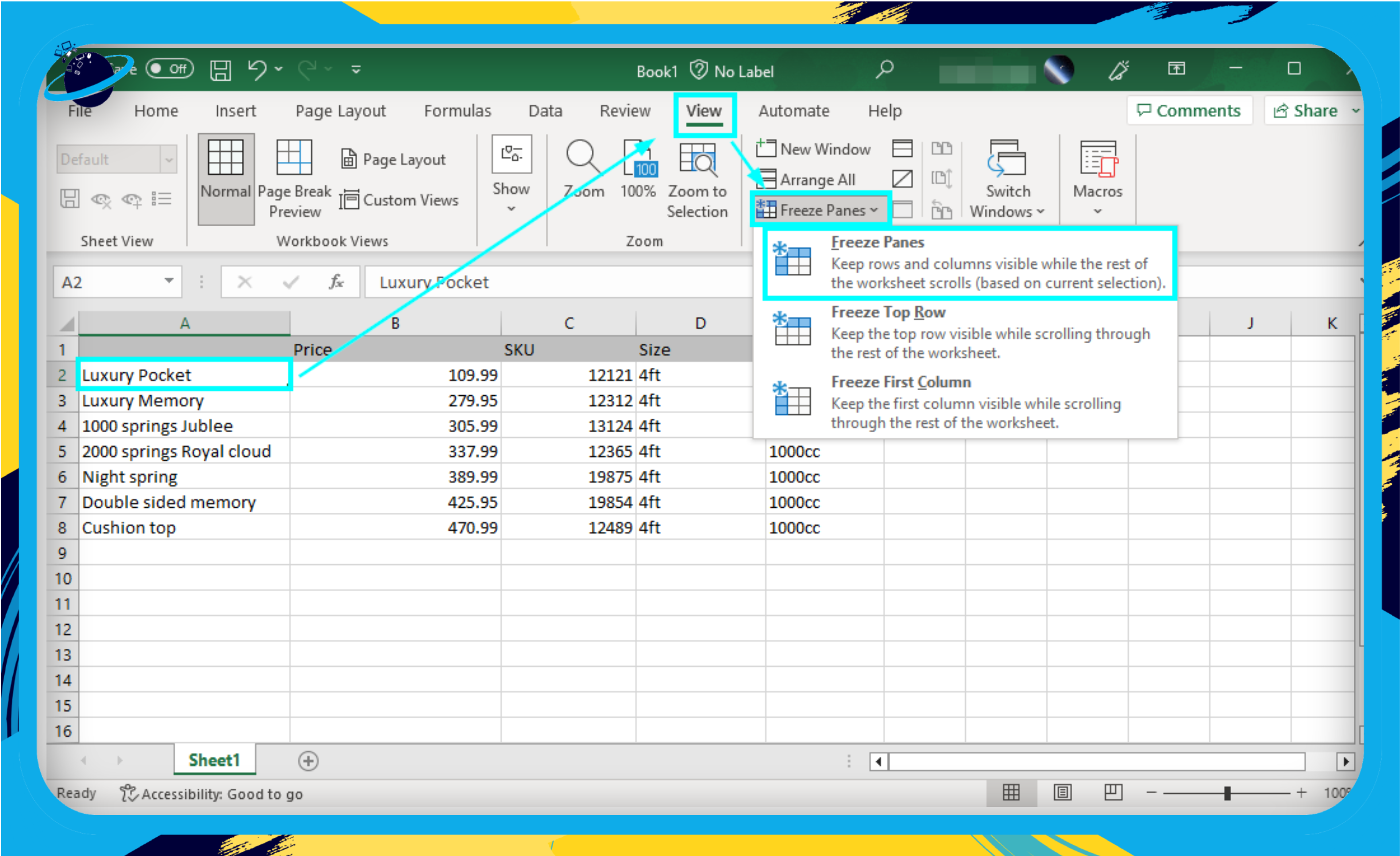
- The “Freeze Panes” Option: This tool enables you to secure rows and columns in your Excel document as required. If you need to freeze the first few rows, the “Freeze Panes” method is handy. Just put a marker under the final row you wish to freeze, go to “View” option, then click on “Freeze Panes”. This action will freeze your chosen rows.
- The “Split” Option: This creates a viewing pane where your added marker will freeze the row from the marked point. It’s another efficient way to freeze rows in Excel.
- How to freeze more than one row in Excel using the “Freeze panes” option.
- How to freeze more than one row in Excel using the “Split” option.
Here are the two methods you can use to help freeze more than one row in Excel. The first method will freeze rows and columns based on what you require, so it is easier to just freeze multiple rows if necessary. The second method will freeze and create additional panes when you are using it. You can go through each one progressively to see which method will work best for you.
How to freeze more than one row in Excel using the “Freeze panes” option
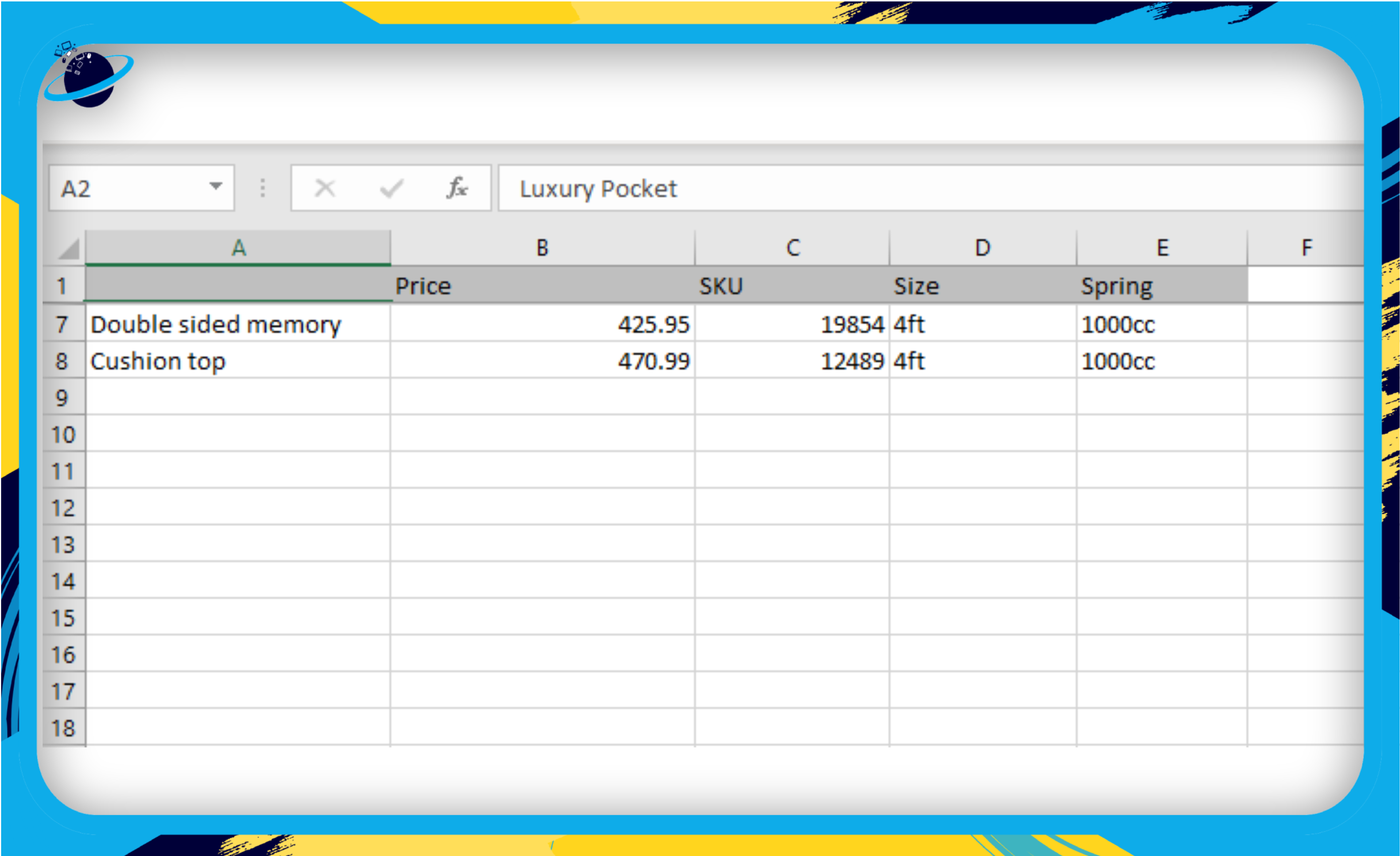
The first method for freezing multiple rows in Excel is the “Freeze Panes” option. With Freeze Panes, you can lock as many rows as you want so that they stay in place while you scroll through the worksheet. Users like to use the Freeze Panes option to create a stationary header or a column that they can use to add important information that they need to be visible at all times.
Please continue reading for the complete steps on how to use the “Freeze panes” option to freeze more than one row in Excel.
- Firstly, open your worksheet in the web or desktop version of Excel.
- Select a row beneath the rows you want to freeze.
- Now click on the option for “View.”
- Click on “Freeze panes” to complete the process.
After following the correct steps, you can freeze rows above the row you’ve chosen. Remember these important points:
- Always select the row below the last one you want to freeze. If you choose the row above, not all rows will be frozen.
- To freeze just the rows, pick the entire row beneath the final one you want to freeze. Selecting a single cell instead of the entire row will also freeze a column.
- To prevent accidental column freezing, ensure you’ve selected the whole row before applying the “Freeze panes” function.
![]() Read More: To learn how yo freeze rows and columns at the same time, read our guide…
Read More: To learn how yo freeze rows and columns at the same time, read our guide…![]() How to freeze top row and the first column at the same time in Excel
How to freeze top row and the first column at the same time in Excel
How to freeze more than one row in Excel using the “Split” option
A lesser-known way to freeze rows in Microsoft Excel is to use the split option within the program. The “Freeze panes” option is the main option many users like to use when they want to freeze rows in Excel. However, the Split option will give you a similar result. Splitting the sheet will generate two or more interactive elements on your document. You will then be able to hover around sections of the panes, and whichever section you hover around, it will move, and you can edit information in that section while the other remains frozen. Like the “Freeze panes” option, you must select a mark beneath the cells you want to freeze. Here is a guide on how to use the Split option in Microsoft Excel to freeze rows.
- Firstly, open the worksheet in the desktop version of Excel.
- From there, select a row under the row you want to freeze.
- Now click on the option for “View.”
- Click on “Split” to complete the process.
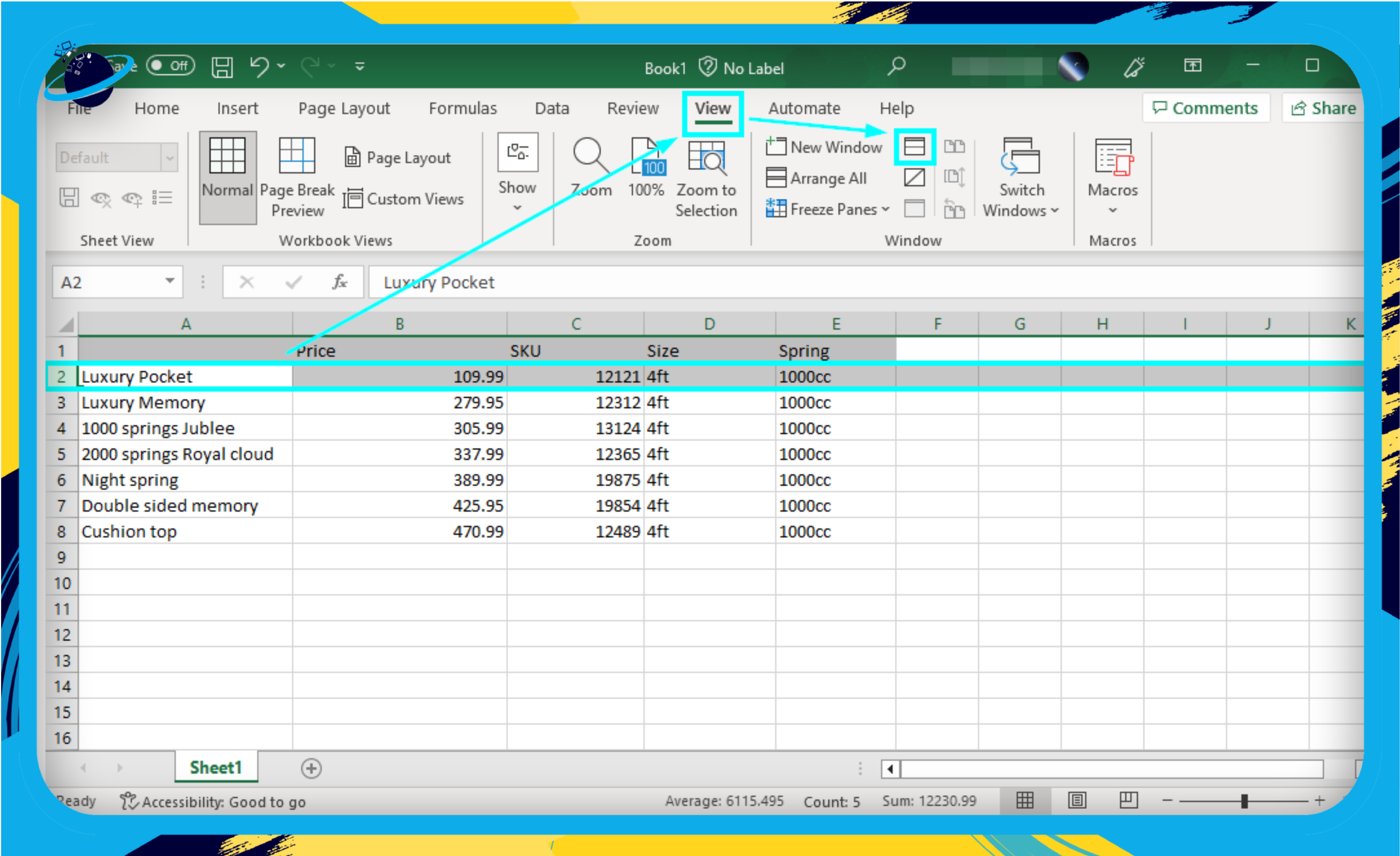
Upon completing the process, you will have managed to split the View from the point you set. The top section will remain frozen until you move your cursor within that zone. You can continue to work on the bottom section, and the rows above will remain frozen until you decide to move your cursor to that zone. Unlike the “Freeze panes” option, you can move the rows; Split will not completely freeze them; however, you will technically have frozen rows as you can work on the section at the bottom without interfering with the rows at the top.
Conclusion
Thank you for reading our blog on freezing multiple rows in an Excel document. I have given you two methods you can use to help freeze rows in Excel. The first method includes the option to use “Freeze panes” to freeze the rows directly. The second option includes splitting the View where you want to freeze the rows. The rows you want to freeze will remain motionless, and you can continue to work on the document in the bottom section. If you encounter any issues following the content, simply drop a comment below, and we will address them.